Why Eigenvalues Lie: Pseudospectra for Non-Normal Operators
math · linear-algebra · numerical-analysis
Claim: In non-normal problems, point eigenvalues are not a reliable diagnostic. You can estimate an operator well (in a norm sense) and still watch its eigenvalues jump all over the complex plane under tiny perturbations.
In data-driven spectral methods—Dynamic Mode Decomposition (DMD), Koopman operators, kernel EDMD—we routinely do the same move: fit an operator from finite data, compute eigenvalues, and read off stability/decay/oscillation as if those points were intrinsic. That move has an implicit assumption:
- Eigenvalues are stable summaries of the operator.
For non-normal operators, that assumption fails. Finite sampling, noise, regularization, truncation—these are not “implementation details”; they are perturbations in , and the map can be hypersensitive.
Pseudospectra are the right object here because they answer the question you actually have in practice: given uncertainty in the operator, where could eigenvalues plausibly be? They replace fragile points with uncertainty-aware regions.
What you’ll get:
- The exact assumption that fails when you “read stability from eigenvalue dots”.
- A concrete perturbation view () and why non-normality amplifies it.
- How pseudospectra turn spectral estimation into set estimation you can trust.
Continuation: If you’re doing Koopman / kernel DMD in practice, the most common downstream failure is spectral pollution—finite-rank projections “invent” modes. Part 2 goes there:
Normal vs. Non-Normal: Where Intuition Breaks
Why are we so easily misled by eigenvalues? Because our intuition is trained on normal operators.
In linear algebra courses, we deal mostly with symmetric or Hermitian matrices (where ) or normal matrices (where eigenvectors are orthogonal). In these safe harbors, eigenvalues are well-conditioned: if you perturb the matrix by a small amount , the eigenvalues move by at most .
But dynamic systems, specifically those governing fluid flow, shear, or transient growth, are rarely normal.
Informally, an operator is non-normal if it does not commute with its adjoint:
The geometric consequence of this inequality is that the eigenvectors of are not orthogonal. They can become nearly parallel, creating a basis that is ill-conditioned. When eigenvectors "lean" on one another, the operator becomes structurally sensitive.
This is not pathological; it is the default in Koopman analysis, EDMD, and any system exhibiting transient growth or shear. In these regimes, the behavior of the system is not dictated solely by the asymptotic fate of eigenvalues. Non-normality does not mean "badly conditioned code"; it is a structural property of the dynamics.
The Eigenvalue Instability Problem
Here is the practical failure mode. In data-driven dynamical systems, you never possess the true operator . You operate on an approximation , derived from finite data, truncated dictionaries, or noisy measurements:
where is a perturbation matrix representing noise or approximation error.
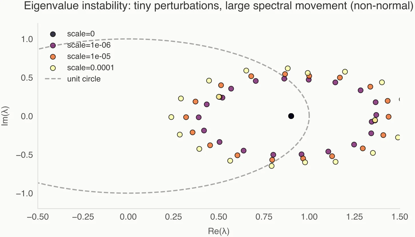
We tend to assume that if the error is small (say, machine precision or modest noise), the eigenvalues of will be close to the eigenvalues of .
In non-normal settings, this logic collapses. Even if is tiny, the eigenvalues of can be wildly different from those of . A stable system (eigenvalues inside the unit disk) can be perturbed by a microscopic amount to yield unstable eigenvalues, or vice versa.
This is often why DMD plots look like "buckshot" scattered across the complex plane, or why Koopman modes struggle to identify true continuous spectra. We are calculating exact eigenvalues of an inexact operator, and the mapping from operator to spectrum is hypersensitive.
Point eigenvalues answer the wrong question: what happens in the limit of zero noise, not what you can trust at finite resolution.
Enter the Pseudospectrum
To fix this, we need to stop looking at points and start looking at regions. We need the pseudospectrum.
The -pseudospectrum of an operator , denoted , is defined as:
In plain English, a complex number is in the pseudospectrum if the resolvent blows up—or, equivalently, if is almost an eigenvalue.
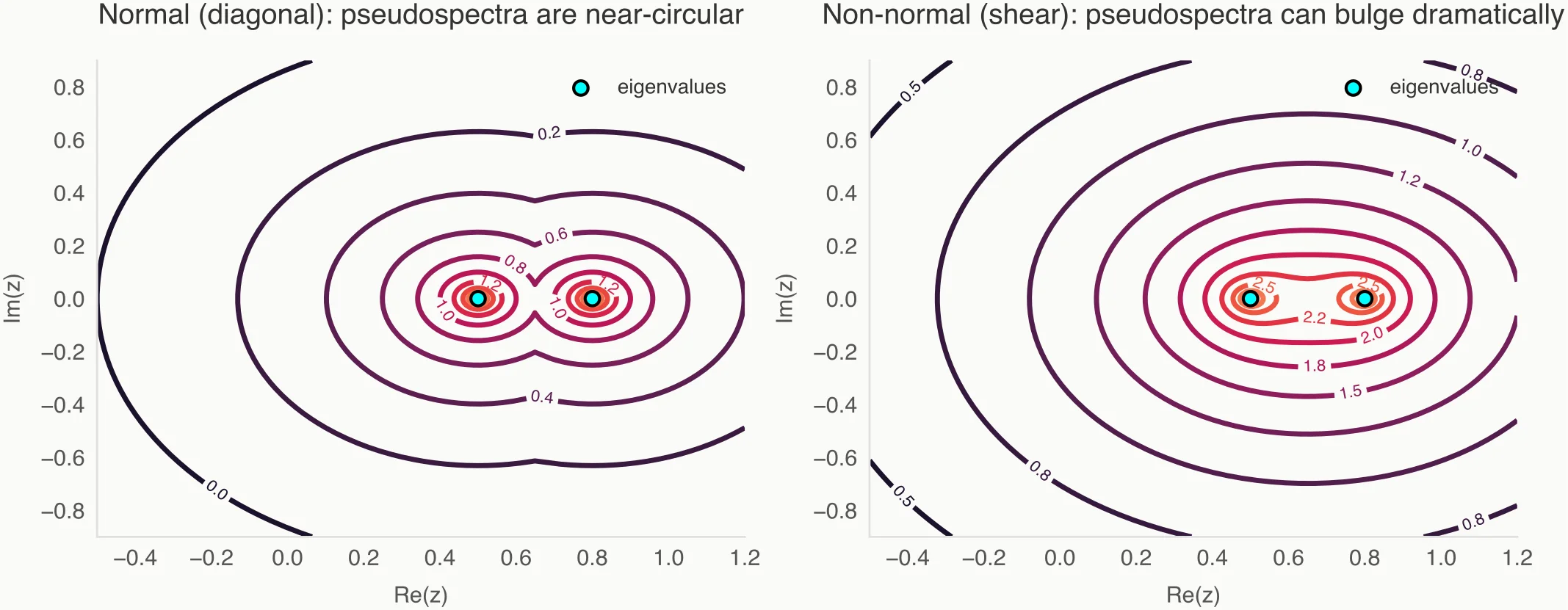
While the traditional spectrum is a set of discrete points (for finite matrices), the pseudospectrum is a set of nested regions (contours) in the complex plane. These regions visualize how "close" the operator is to singularity at any given point .
If the operator is normal, these regions are perfect circular disks of radius around the eigenvalues. But for non-normal operators, these regions can expand dramatically, stretching far away from the eigenvalues, swallowing large portions of the complex plane.
Pseudospectra describe where eigenvalues could plausibly be, given noise and approximation error.
Containment: What Pseudospectra Actually Guarantee
Pseudospectra are not just pretty visualizations; they provide rigorous bounds on spectral uncertainty. This is reframed through the property of containment.
If our approximated operator is close to the true physics within some tolerance (i.e., ), then the following containment holds:
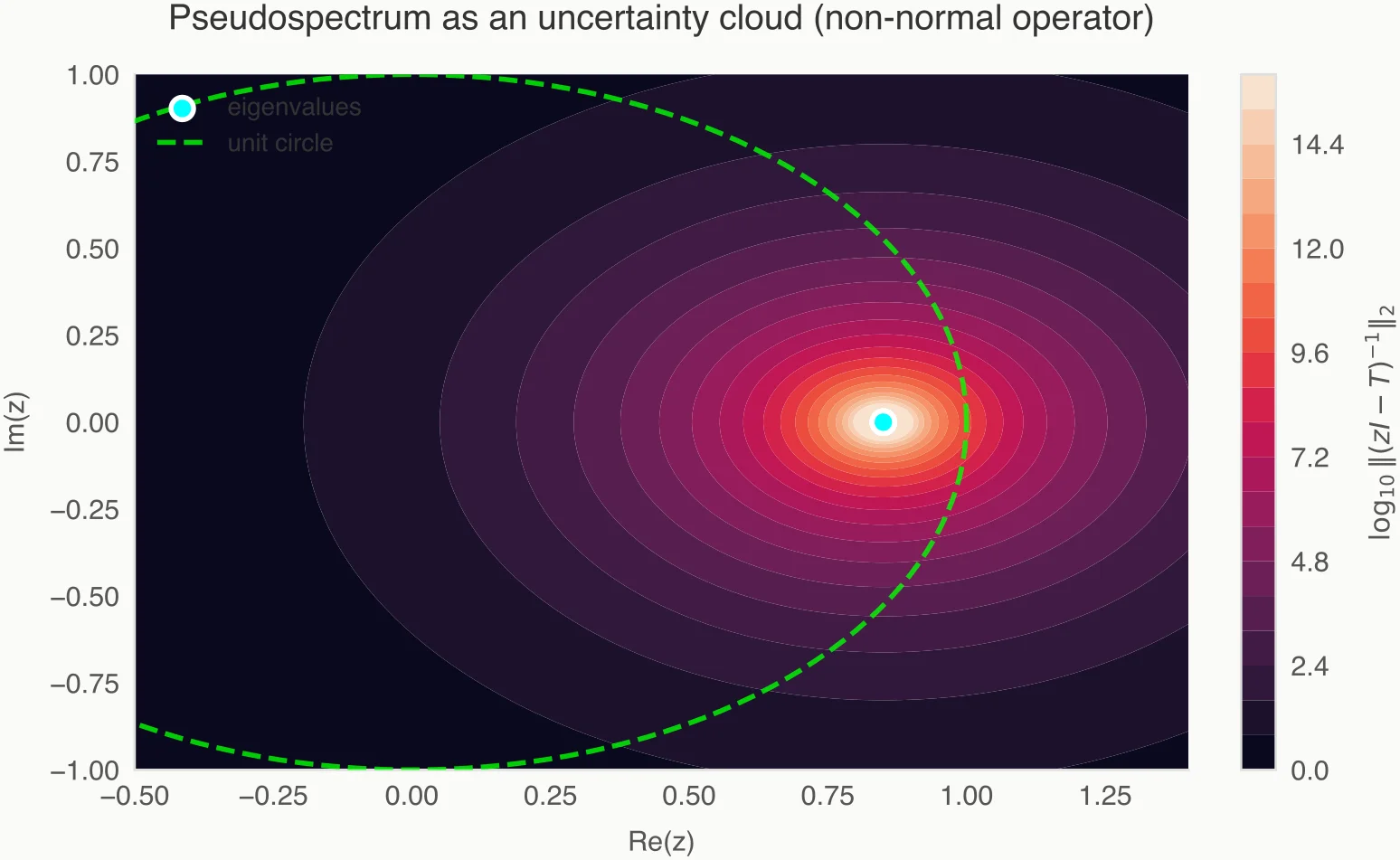
This statement is powerful. It tells us that the true eigenvalues of the unknown system must live somewhere inside the -pseudospectral cloud computed from our data-driven model .
If the pseudospectrum is a tight cluster around a point, you can trust that eigenvalue. If it is a massive, sprawling blob traversing the unit circle, that point eigenvalue you calculated is meaningless. It is merely one possible realization in a vast sea of uncertainty.
This reframes spectral estimation as set estimation. We are no longer hunting for coordinates; we are bounding the region where the physics lives.
Why This Matters for Data-Driven Operators
This perspective is critical for modern applied mathematics, particularly for methods like Extended Dynamic Mode Decomposition (EDMD) and Kernel Koopman approaches.
Consider the workflow of a typical Koopman analysis:
- We project infinite-dimensional dynamics onto a finite subspace.
- We regularize the inverse (e.g., Tikhonov regularization or ridge regression) to handle ill-conditioning.
- We act on noisy data.
Every step here introduces a perturbation .
When you look at a standard eigenvalue plot from EDMD, you are seeing a result that is hypersensitive to the regularization parameter . Change slightly, and the eigenvalues might migrate significantly.

Pseudospectra naturally absorb this uncertainty. They reveal that regularization does not just stabilize inversion; it reshapes the pseudospectrum.
By computing the pseudospectrum, you can distinguish between:
- Spectral features: Regions where the resolvent norm is huge regardless of small perturbations.
- Numerical artifacts: Eigenvalues that exist only for a specific regularization setting but vanish or move wildly when checked against the resolvent.
If you are doing stability analysis on a fluid simulation using DMD, relying on a single unstable eigenvalue to predict onset of turbulence is risky. Relying on the pseudospectrum crossing the stability boundary is robust.
Pseudospectra vs. "Spectral Pollution"
One of the greatest enemies in infinite-dimensional operator approximation is spectral pollution—spurious eigenvalues that arise purely from the discretization process.
In Galerkin projections (used in EDMD), we often see eigenvalues appearing in gaps of the continuous spectrum. These are "numerical mirages." A standard eigen-solver cannot distinguish between a physical mode and a discretization artifact.
Pseudospectra provide the filter.
- A true eigenvalue usually sits at the bottom of a deep pseudospectral "well."
- Spectral pollution often appears as a shallow dimple in the resolvent surface.
A point eigenvalue without a surrounding pseudospectral basin is a numerical mirage. By thresholding the resolvent norm, we can effectively scrub these pollutants from our model, leaving only the structurally stable dynamics.
Practical Guidance
So, how do you change your workflow? You do not need to abandon eigenvalues, but you must validate them.
When to trust eigenvalues:
- They are isolated from the rest of the spectrum.
- They are surrounded by tight, concentric pseudospectral contours.
- The norm of the resolvent is massive at that location.
When to be skeptical:
- Eigenvalues appear in dense clusters or lines (indicating a discretized continuous spectrum).
- The eigenvalues move dramatically when you change the regularization parameter or resample the data.
- The pseudospectral contours are elongated, suggesting that a small perturbation could push the eigenvalue across the imaginary axis (or unit circle).
The Next Step: Stop plotting dots. Start plotting contours of . It is computationally more expensive, but for high-stakes modeling, it is the only way to know if your stability analysis is real or a numerical fiction.
Conclusion — Changing the Mental Model
We need to retire the idea that a dynamical system—especially a data-driven one—can be summarized by a list of precise complex numbers.
Spectral estimation in non-normal problems should be thought of as estimating regions, not points.
By adopting pseudospectra, we move away from false precision and toward honest modeling. We explicitly acknowledge the uncertainty inherent in our finite, noisy data and visualize it. This does not weaken our results; it strengthens them, ensuring that the dynamics we claim to discover are features of the physics, not flaws in our linear algebra.