The Magic of Morphing Math: A Deep Dive into Normalizing Flows

In the world of generative modeling, we often face a daunting challenge: how do we teach a computer to understand and recreate the messy, complex distributions of the real world? Whether it's the distribution of pixels in a human face or the structural patterns of a protein, the underlying "probability density" is incredibly intricate.

Enter Normalizing Flows. As a mathematician, I find these models particularly elegant because they don't just approximate data—they transform it. By using the fundamental principles of calculus and geometry, Normalizing Flows allow us to morph a simple Gaussian "blob" into a complex data manifold and back again.

1. The Core Philosophy: Simplicity to Complexity

The central idea is to model a complex data distribution by transforming a simple, well-defined base distribution (usually a standard multivariate Gaussian).

We define a deterministic and invertible function such that:

Because is invertible, we can also go backward: . This invertibility is the "secret sauce" that allows us to evaluate the density of our data exactly.

1.1 The Change of Variables Formula

To relate the density of our complex data to our simple latent space, we use the Change of Variables Formula. If is invertible and differentiable, the relationship between densities is:

Here, is the Jacobian of the inverse transformation. The determinant of the Jacobian accounts for how the transformation stretches or compresses the "volume" of space. If the function pulls points apart, the density decreases; if it pushes them together, the density increases.

1.2 Training via Log-Likelihood

In practice, we don't maximize the likelihood directly because multiplying thousands of small probabilities leads to numerical underflow. Instead, we use the Log-Likelihood:

Why the Logarithm?

• Numerical Stability: It turns products into sums, preventing our computers from rounding small values to zero.
• Easier Optimization: The logarithm is monotonic. Maximizing the log-likelihood is mathematically equivalent to maximizing the likelihood itself.
• Gradient Friendly: Sums are much easier to differentiate than products, making backpropagation significantly more efficient.

2. Building Deep Flows: The Power of Composition

A single simple transformation isn't enough to capture the nuance of a "Two-Moons" dataset, let alone an image. However, the composition of multiple invertible functions is itself invertible.

If we have layers:

The log-determinant of the total Jacobian is simply the sum of the log-determinants of each layer:

This additive property is a computational lifesaver. It allows us to stack simple layers to build a "deep" flow without the math becoming intractable.

3. Real NVP: The Architect's Choice

One of the most influential flow architectures is Real NVP (Real-valued Non-Volume Preserving). It uses Coupling Layers to ensure the Jacobian is easy to calculate while remaining highly expressive.

The Coupling Mechanism

The input vector is split into two halves, and .

1. Identity Part: (stays the same).
2. Transformed Part: .

The functions (scale) and (bias) can be any complex neural network. They don't need to be invertible themselves because we only ever evaluate them on the identity part .

The Genius of the Jacobian:

Because doesn't depend on , and depends on only element-wise, the Jacobian matrix becomes lower triangular. The determinant of a triangular matrix is just the product of its diagonal elements.

This makes the computation of the volume change incredibly fast!

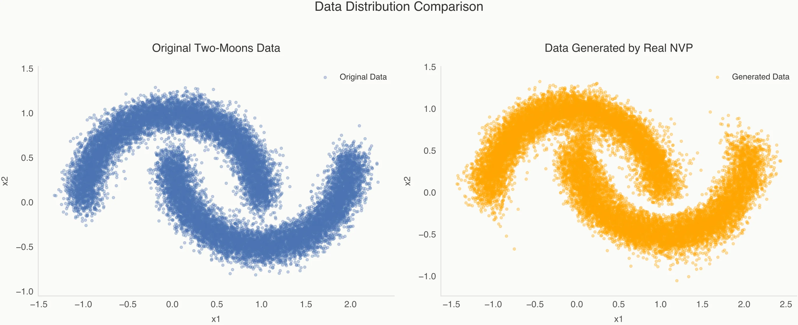
4. Seeing it in Action: The "Two-Moons" Experiment

To prove the power of this math, let's look at a Python implementation using PyTorch. We want to see if our model can learn to turn a circular Gaussian distribution into two interlocking crescents.

import torch
import torch.nn as nn

class CouplingLayer(nn.Module):
    def __init__(self, data_dim, hidden_dim, mask):
        super().__init__()
        self.mask = mask
        # Neural networks for scale and bias
        self.s_net = nn.Sequential(nn.Linear(data_dim, hidden_dim), nn.ReLU(), 
                                   nn.Linear(hidden_dim, data_dim))
        self.b_net = nn.Sequential(nn.Linear(data_dim, hidden_dim), nn.ReLU(), 
                                   nn.Linear(hidden_dim, data_dim))

    def forward(self, z):
        z_a = z * self.mask
        s = self.s_net(z_a)
        b = self.b_net(z_a)
        x = z_a + (1 - self.mask) * (z * torch.exp(s) + b)
        log_det_J = ((1 - self.mask) * s).sum(dim=1)
        return x, log_det_J

    def inverse(self, x):
        x_a = x * self.mask
        s = self.s_net(x_a)
        b = self.b_net(x_a)
        z = x_a + (1 - self.mask) * ((x - b) * torch.exp(-s))
        log_det_J_inv = ((1 - self.mask) * -s).sum(dim=1)
        return z, log_det_J_inv

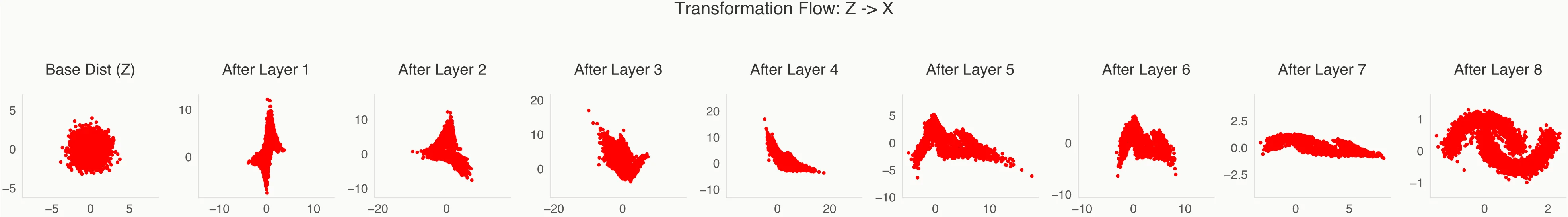
The Evolution of a Distribution

The beauty of Normalizing Flows is that we can "peek" inside the model to see how the data evolves through each layer. Initially, the points are clustered in a standard normal "blob" (). As they pass through successive layers, the space is stretched, folded, and shifted.

Figure 1: The visual evolution of the "Transformation Flow." Each subplot represents the state of the data distribution after passing through a specific layer. Notice how the initial Gaussian is gradually molded into the distinct "Two-Moons" shape by Layer 8.

Analysis of the Flow

• Layers 1-3: The model begins by breaking the symmetry of the Gaussian, pulling the distribution into an elongated shape.
• Layers 4-6: The "coupling" effect becomes visible as the model starts to "bend" the distribution, creating the hollow space between the two crescents.
• Layers 7-8: The final layers refine the boundaries and ensure the density perfectly matches the training data.

The Result: From Chaos to Order

After training for 1000 epochs, the transformation is mesmerizing. We start with a standard normal distribution in the latent space () and watch as each layer of the flow warps, stretches, and bends the space until it perfectly matches the "Two-Moons" data ().

• Training Loss: We observed the negative log-likelihood drop from initial noise to a stable point around 1.01.
• Generation: To create new data, we simply sample from the Gaussian and run the "forward" pass. The model creates "moons" that are indistinguishable from the training set.

Conclusion

Normalizing Flows represent a beautiful intersection of rigorous mathematics and deep learning. By enforcing invertibility and tracking volume changes via the Jacobian, we gain the ability to evaluate exact probability densities—something Generative Adversarial Networks (GANs) simply cannot do.

Whether you are interested in physics-informed machine learning or high-fidelity image generation, "the flow" offers a mathematically grounded path forward.

Would you like me to dive deeper into the specific neural network architectures used for the scale and bias functions, or perhaps explain how we can use these for anomaly detection?